
At moderate volumes, AWS Glue feels almost effortless.
You increase workers. The job runs faster.
You double the input size. Runtime roughly doubles.
Everything behaves predictably.
Then one day, it stops behaving that way.
We had a job that ran in about 15 minutes. The dataset grew. Runtime climbed to 27. That made sense. We increased workers. It dropped to 22.
We increased workers again.
It dropped to 21.
That was the moment it became clear we weren’t compute-bound anymore.
What slowed the job down wasn’t CPU. It wasn’t memory. It wasn’t even S3 read time.
It was shuffle. It was skew. And it was file behavior.
This article walks through the experiments I ran to understand where Glue jobs really break at scale — and what actually fixes them.
The Setup
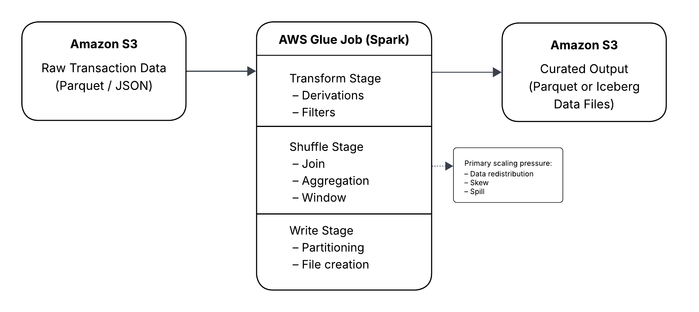
The pipeline is simple.
Raw transaction-style data lands in S3.
A Glue job transforms it, joins it to a small dimension table, aggregates it, and writes the result back to S3.
Sometimes the output is plain Parquet. Sometimes it’s written to Iceberg.
No streaming. No ML. No exotic orchestration.
Just Spark running inside Glue.
To keep this reproducible, I generated synthetic data inside Spark.
from pyspark.sql import functions as F

def generate_transactions(rows: int):
    return (
        spark.range(rows)
            .withColumnRenamed("id", "txn_id_num")
            .withColumn("account_id",
                (F.col("txn_id_num") % 500000).cast("string")
            )
            .withColumn("amount", (F.rand(42) * 500).cast("double"))
            .withColumn(
                "txn_ts",
                F.expr("""
                    timestampadd(
                        MINUTE,
                        cast(txn_id_num % 100000 as int),
                        timestamp('2025-01-01 00:00:00')
                    )
                """)
            )
            .withColumn("txn_date", F.to_date("txn_ts"))
            .withColumn("merchant_code",
                (F.col("txn_id_num") % 10000).cast("int")
            )
            .drop("txn_id_num")
    )
This lets us scale from 5 million rows to hundreds of millions without introducing unknown variables.
Where a Glue Job Can Actually Slow Down
Before going deeper, it helps to anchor the discussion in how a Glue job actually executes.
Most Glue job performance issues map cleanly to one of five phases:
- Read from S3
- Transform
- Shuffle
- Write
- Commit metadata (optional)
When Scaling Still Works
The first experiment was intentionally simple.
df = generate_transactions(50_000_000)

df_baseline = (
    df.withColumn("amount_bucket",
        F.when(F.col("amount") < 50, "LOW")
         .when(F.col("amount") < 200, "MED")
         .otherwise("HIGH")
    )
    .groupBy("txn_date")
    .agg(F.count("*").alias("txn_cnt"))
)
At 5 million rows, the job was quick.
At 50 million, runtime increased proportionally.
At 200 million, it was slower but still predictable.
This is what Spark does well: narrow transformations and simple aggregations scale cleanly.
The problems start when the workload becomes wide.
The Shuffle Shift
Things changed as soon as I introduced a join and grouped by a higher-cardinality key.
dim = (
    spark.range(0, 10000)
        .withColumnRenamed("id", "merchant_code")
        .withColumn("merchant_category",
            F.concat(F.lit("cat_"), (F.col("merchant_code") % 50))
        )
)

df_joined = df.join(dim, "merchant_code", "left")

df_agg = (
    df_joined.groupBy("txn_date", "merchant_category")
        .agg(
            F.count("*").alias("txn_cnt"),
            F.sum("amount").alias("total_amount")
        )
)
Runtime increased, but what mattered more was what the Spark UI showed.
Most of the time was now spent inside shuffle stages.
CPU wasn’t pegged.
Executors weren’t maxed out.
But the shuffle stage consumed the majority of runtime.
That distinction matters.
When a job is compute-bound, adding workers usually helps.
When a job is shuffle-bound, the bottleneck shifts to data movement.
Shuffle is not just another transformation. It is full data redistribution across the cluster. Rows are repartitioned by key, exchanged across executors, and often written to disk before being merged again.
It is network-heavy.
It is disk-heavy.
And it is extremely sensitive to key distribution and imbalance.
Once shuffle dominates runtime, adding workers produces diminishing returns.
Why?
Because you are no longer limited by raw compute. You are limited by how evenly data can be distributed across partitions.
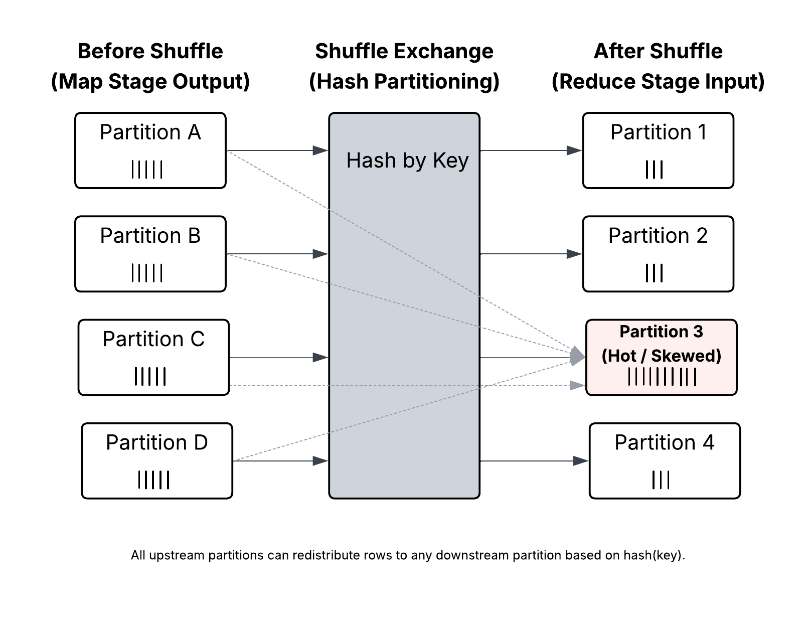
Skew: The Silent Runtime Killer
To test skew, I ran:
df.groupBy("account_id")
  .count()
  .orderBy(F.desc("count"))
  .show(10)
A few keys had dramatically more rows than others.
That explains long-running tasks at the tail of shuffle stages.
Distributed systems are only as parallel as their most overloaded partition.
One partition holding millions of rows can stall the entire stage.
Salting as a Controlled Tradeoff
One mitigation is salting:
salted = df.withColumn("salt", (F.rand() * 10).cast("int"))

salted = salted.withColumn(
    "account_salted",
    F.concat_ws("_", "account_id", "salt")
)
This spreads large keys across partitions.
It improves parallelism.
It also increases shuffle complexity and requires careful downstream handling.
Salting is a tradeoff, not a universal fix.
The Partitioning Trap
The most dramatic slowdown wasn’t from shuffle. It was from partitioning.
Partitioning by txn_date behaved well.
Partitioning by account_id looked logical. It wasn’t.
df.write
  .mode("overwrite")
  .partitionBy("account_id")
  .parquet("s3://bucket/account_partition/")
The result:
- File counts exploded
- Write time increased significantly
- Average file size dropped sharply
High-cardinality partitioning multiplies partitions and files.
Each Spark task can write one file per partition. At scale, that becomes thousands of files.
Small Files Are Not Harmless
Small files affect:
- S3 object listing
- Query planning
- Metadata operations
- Compaction requirements
The fix is not random repartitioning.
It’s intentional shaping.
df.repartition(200, "txn_date")
  .write.partitionBy("txn_date")
  .parquet("...")
Aligning repartitioning with partition columns reduces file chaos.
When Iceberg Enters the Picture
Writing plain Parquet exposes file-level problems.
Writing to Apache Iceberg adds a metadata layer.
Each write creates:
- Data files
- Manifest entries
- A snapshot
- A commit operation
If file counts are high, commit time grows.
If partitions are excessive, manifest lists expand.
Creating the table is straightforward:
CREATE TABLE transactions_iceberg (
    txn_id STRING,
    account_id STRING,
    txn_ts TIMESTAMP,
    amount DOUBLE
)
USING iceberg
PARTITIONED BY (days(txn_ts));
Writing is equally simple:
df.repartition(200, "txn_date")
  .writeTo("catalog.db.transactions_iceberg")
  .append()
The complexity shows up later:
- Slower planning
- Growing snapshot history
- Metadata overhead that scales with file count
Iceberg doesn’t create performance issues. It amplifies poor file discipline.
The Serverless Ceiling
There is a point where:
- Shuffle dominates runtime
- Skew stalls a subset of tasks
- File creation dominates write time
- Commit time becomes visible
- Increasing workers has minimal effect
At that point, the scaling curve flattens.
That’s the serverless ceiling.
Adding more workers doesn’t help.
Reshaping the workload does.
Reducing shuffle width.
Managing skew.
Designing sane partition strategies.
Controlling file size intentionally.
Those changes moved runtime more than any worker increase did.
Closing Thought
Serverless removes cluster management. It does not remove distributed systems physics.
Data movement still costs.
Imbalance still hurts.
Files still matter.
Metadata still accumulates.
Once you start thinking in terms of workload shape instead of raw compute, Glue scaling becomes much more predictable.
And the next time a job jumps from 15 minutes to 40, you’ll know exactly where to look.

![How to Use FTP to Upload Files to WordPress Without Password [Step By Step]](https://wiredgorilla.com.au/wp-content/uploads/2025/04/how-to-use-ftp-to-upload-files-to-wordpress-without-password-step-by-step-768x348.png)