What is Clustering
Clustering is a type of unsupervised machine learning technique that groups similar data points together. Clustering helps you automatically identify patterns or natural groups hidden in your data.
Imagine this scenario:
You’ve recently launched an e-commerce platform that sells pre-portioned meals and recipes. Different types of customers lean toward different kinds of meals. Younger customers may prefer lower-cost, single-serving meals. People in their 30s may be shopping for two and often opt for organic upgrades. Customers over 50 might need meals tailored around specific dietary needs, such as diabetic-friendly choices.
At first glance, these seem like straightforward clusters. But once you factor in additional variables, such as income, location, and festive seasons, the patterns become far more complex.
Dataset
Online Retail Data Set (UCI): Transactional data for market segmentation
https://www.kaggle.com/datasets/vijayuv/onlineretail
This dataset contains a transactional log of purchases made by customers from an online retail store. It provides detailed invoice-level information about products sold over a specific time period.
K-Means Algorithm Overview
K-means is a popular clustering algorithm due to its simplicity, speed, and effectiveness in partitioning large datasets into distinct groups based on feature similarity. It works by minimizing the distance between data points and their assigned cluster centers (centroids).
When is K-means Used
- To discover natural groupings in unlabeled data
- When the data is numeric and clusters are expected to be roughly spherical and similar in size
Common applications: customer segmentation, market analysis, image compression, anomaly detection, and pattern recognition.
K-means is ideal when we need scalable, interpretable clustering and your data aligns with its assumptions.
K-Means Algorithm Steps
- Choose the number of clusters (k)
- Randomly initialize k centroids in d-dimensional space
- Assign each data point to the nearest centroid (using Euclidean distance)
- Move each centroid to the mean of its assigned points
- Repeat steps 3-4 until cluster assignments stabilize.
Assumptions
- Clusters are spherical and equally sized
- Data is numeric and scaled
Important: K-means clustering uses Euclidean distance to assign points to clusters. If features are on different scales (e.g., price vs. quantity), those with larger ranges will dominate the distance calculation, producing biased clusters. Feature scaling ensures all features contribute equally, resulting in meaningful and balanced clusters.
Data Preprocessing
- Handle missing values
- Remove or cap outliers
- Scale features
import pandas as pd
import numpy as np
import matplotlib.pyplot as plt
import seaborn as sns
from sklearn.cluster import KMeans
from sklearn.preprocessing import StandardScaler

#/Users/raja.chakraborty/Downloads/OnlineRetail.csv
df = pd.read_csv('/Users/raja.chakraborty/Downloads/OnlineRetail.csv', nrows=30000)
# 30k to speed up things
print(df.shape)
print(df.head())


output
(30000, 8)
  InvoiceNo StockCode                          Description  Quantity
0    536365    85123A   WHITE HANGING HEART T-LIGHT HOLDER         6
1    536365     71053                  WHITE METAL LANTERN         6
2    536365    84406B       CREAM CUPID HEARTS COAT HANGER         8
3    536365    84029G  KNITTED UNION FLAG HOT WATER BOTTLE         6
4    536365    84029E       RED WOOLLY HOTTIE WHITE HEART.         6

      InvoiceDate  UnitPrice  CustomerID         Country
0  12/1/2010 8:26       2.55     17850.0  United Kingdom
1  12/1/2010 8:26       3.39     17850.0  United Kingdom
2  12/1/2010 8:26       2.75     17850.0  United Kingdom
3  12/1/2010 8:26       3.39     17850.0  United Kingdom
4  12/1/2010 8:26       3.39     17850.0  United Kingdom
Data Exploration
Begin by checking for missing values, outliers, and incorrect datatypes, followed by visual distribution checks.
print(df.info())
print(df.describe())
sns.boxplot(data=df)
plt.show()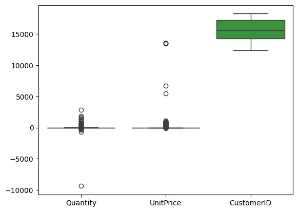
From the box plot, we can clearly see outliers. We’ll handle this using IQR-based treatment capping. Note that CustomerId has no outliers, so it remains unaffected by this treatment.
Finding Optimal k (Elbow Method)
Choose k where the inertia curve bends (“elbow”).
inertia = []
K = range(1, 11)
for k in K:
    kmeans = KMeans(n_clusters=k, random_state=42)
    kmeans.fit(X_scaled)
    inertia.append(kmeans.inertia_)

plt.plot(K, inertia, 'bx-')
plt.xlabel('Number of clusters')
plt.ylabel('Inertia')
plt.title('Elbow Method For Optimal k')
plt.show()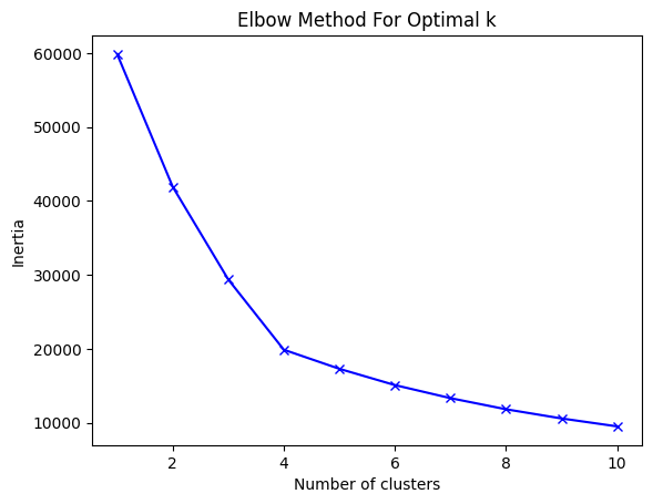
We selected K=4, as the elbow curve begins to bend noticeably at that point, indicating an optimal number of clusters. While outliers beyond K=6 could pose challenges, choosing 4 provides a balanced and practical clustering solution for the dataset.
optimal_k = 4
kmeans = KMeans(n_clusters=optimal_k, random_state=42)
clusters = kmeans.fit_predict(X_scaled)
df['Cluster'] = clusters

sns.pairplot(df, hue='Cluster')
plt.show()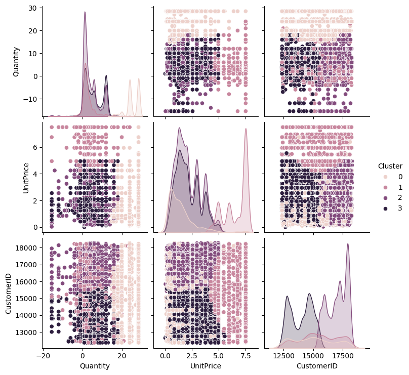
As per the above pair plot, K=4 offers clean separation and meaningful groupings.
What Are the Main Customer Segments in the Retail Dataset
The clusters reveal distinct segments such as bulk buyers, budget shoppers, premium customers, and standard retail customers. These insights can help tailor marketing strategies and product offerings for each segment.
How Do Clusters Differ
Each cluster varies in average quantity, unit price, and other transaction features, highlighting differences in purchasing behavior. For example, bulk buyers may respond better to volume discounts, while premium customers may value exclusive products.
Minimizing Variation
Model Validation
To validate cluster quality, we used the silhouette score.
from sklearn.metrics import silhouette_score
score = silhouette_score(X_scaled, clusters)
print(f'Silhouette Score: {score:.2f}')

output

Silhouette Score: 0.38Interpretation:
- Values close to 1 indicate well-separated, dense clusters.
- Values near 0 mean clusters overlap or are not well-defined.
- Values below 0 suggest points may be assigned to the wrong cluster.
Our model scored 0.38, indicating reasonable clustering with some overlapping behavior (expected for real-world retail data). While we experimented with different values of K (such as 2, 3, 5, and 6), none of them resulted in better performance or clearer groupings compared to K=4. This could be because of the underlying characteristics of the dataset.
Cluster Characteristics Summary
After applying K-means clustering with k=4, each cluster represents a distinct group of customers based on their purchasing behavior and transaction attributes. By analyzing the cluster centers and feature distributions, we observe the following:
- Cluster 0: Customers in this group tend to have higher average quantities per transaction and moderate unit prices. This may represent bulk buyers or wholesale customers.
- Cluster 1: This cluster is characterized by lower quantities and lower unit prices, possibly indicating occasional or budget-conscious shoppers.
- Cluster 2: Customers here show high unit prices but lower quantities, suggesting premium product buyers or those purchasing expensive items in small amounts.
- Cluster 3: This group has moderate quantities and unit prices, likely representing typical retail customers with standard purchasing patterns.
Limitations and improvements
For use cases like a meal-prep platform, clustering helps tailor meal recommendations to different user segments, improving personalization and customer satisfaction.
While K-Means offers a solid starting point, exploring alternative algorithms like DBSCAN and optimizing for scale will ensure the system remains accurate, flexible, and efficient as your user base grows.